11.3 – Implementing a linear 2-class SVM

Before we proceed to look at the case where the data is not linearly separable, let’s first solidify the foundations of SVMs by implementing an SVM. Our SVM will not have a kernel (also called a linear kernel), and will use a convex optimization library. Recall that the SVM problem is a quadratic programming problem (QPP). Our convex optimization library of choice will be cvxopt.

A lot of the code in this blog post was taken from this blog post by Xavier Bourret Sicotte. Plotting the decision boundary is code taken from here.

Let’s start by making a dataset and ensuring it’s linearly separable.

from sklearn.datasets import make_blobs
import matplotlib.pyplot as plt
import numpy as np

plt.style.use('ggplot')

X, y = make_blobs(n_samples=1000, centers=2,
                  n_features=2, random_state=1)

y[y == 0] = -1

The last line changes the 0s to -1, since that is what our mathematical framework assumes. Let’s visualize this data.

plt.xlabel('$x_1$')
plt.ylabel('$x_2$')
plt.scatter(X.T[0], X.T[1], c=y+1, alpha=0.3);

For convenience, let’s give y a 2D shape rather than let it be a rank-one tensor. Let’s multiply all the values with 1.0 (a float) to force all the values to be floating-points.

y = y.reshape(-1, 1) * 1.

Now it’s time to frame our dual problem and solve it using the convex optimization library. There is a rather technical problem, however. You see, our dual problem is posed as:

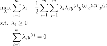
$\begin{aligned} \max\limits_{\boldsymbol\lambda} & \sum\limits_{i=1}^m \lambda_i - \frac{1}{2}\sum\limits_{i=1}^m \sum\limits_{j=1}^m \lambda_i \lambda_j y^{(i)}y^{(j)} x^{(i)T}x^{(j)} \\ \text{s.t. } & \lambda_i \geq 0 \\ & \sum\limits_{i=1}^m \lambda_i y^{(i)} = 0 \end{aligned}$

However, cvxopt expects a QPP of the form

$\begin{aligned} & \min \frac{1}{2} x^TPx + q^Tx \\ \text{s.t. } & Gx \leq h \\ & \ Ax = b \end{aligned}$

Xavier’s blog post shows a clever trick: let’s first begin by forming a matrix $H$ such that

$H_{ij} = y^{(i)}y^{(j)}x^{(i)T}x^{(j)}$

Then, our dual problem becomes

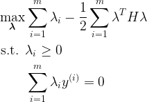
$\begin{aligned} \max\limits_{\boldsymbol\lambda} & \sum\limits_{i=1}^m \lambda_i - \frac{1}{2}\sum\limits_{i=1}^m \lambda^T H \lambda \\ \text{s.t. } & \lambda_i \geq 0 \\ & \sum\limits_{i=1}^m \lambda_i y^{(i)} = 0 \end{aligned}$

We’re not quite there yet. We need a min instead of a max, and a change of sign in the constraint. The trick is easy: for the first issue, we simply take the negative of the optimization problem. Maximizing something is equivalent to minimizing its negative. For the second issue, we also do the same thing. Thus, the optimization problem we give the library is

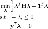
$\begin{aligned} \min\limits_{\boldsymbol\lambda} & \frac{1}{2}\boldsymbol\lambda^T \textbf{H}\boldsymbol\lambda - \textbf{1}^T \boldsymbol\lambda \\ \text{s.t. } & -\lambda_i \leq 0 \\ & \textbf{y}^T \boldsymbol\lambda = 0 \end{aligned}$

Let’s note the correspondence between these two problems:

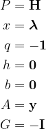
$\begin{aligned} P &= \textbf{H} \\ x &= \boldsymbol\lambda \\ q &= -\textbf{1} \\ h &= \textbf{0} \\ b &= \textbf{0} \\ A &= \textbf{y} \\ G &= -\textbf{I} \end{aligned}$

We can now import the convex optimization library and convert our data to its format, and ask it to solve the QP problem for us.

from cvxopt import matrix as cvxopt_matrix
from cvxopt import solvers as cvxopt_solvers

m, n = X.shape
X_dash = y * X
H = np.dot(X_dash, X_dash.T) * 1.
P = cvxopt_matrix(H)
q = cvxopt_matrix(-np.ones((m, 1)))
h = cvxopt_matrix(np.zeros(m))
A = cvxopt_matrix(y.reshape(1, -1))
b = cvxopt_matrix(np.zeros(1))
G = cvxopt_matrix(-np.eye(m))

cvxopt_solvers.options['show_progress'] = False
sol = cvxopt_solvers.qp(P, q, G, h, A, b)

Noting the correspondence, we know this solution has $\lambda$ . Let’s grab that.

lambd = np.array(sol['x'])

Using equation 1 from our previous post, let’s compute $w$ .

w = ((y * lambd).T @ X).reshape(-1,1)

Finally, let’s use the equation for $b^*$ from the previous post to get $b$ (this is different from Xavier’s blog post, but the end result is the same).

ind = np.where(y == -1)[0]
p1 = X[ind] @ w

ind = np.where(y == 1)[0]
p2 = X[ind] @ w

b = (max(p1) + min(p2)) / 2

We’re done! If you print out $w$ and $b$ , you should get $b = 1.352, w=[-0.233, -0.269]$ .

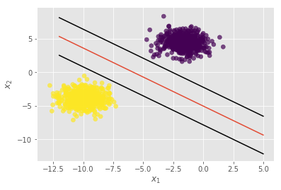
Let’s plot the decision boundary.

plt.xlabel('$x_1$')
plt.ylabel('$x_2$')

xx = np.linspace(-12, 5)
slope = -w[0] / w[1]
intercept = b / w[1]
yy = slope * xx + intercept
plt.plot(xx, yy, 'k-')

plt.scatter(X.T[0], X.T[1], c=y.squeeze()+1, alpha=0.7);

index1

We can even plot the support vectors (although why they don’t actually pass through one point on each side, I’m not sure). The key idea is that the width of the margin of the SVM is $\frac{1}{\left\Vert w \right\Vert}$ , on each side (you should be able to see this from our formulation in the initial SVM blog post). The additional lines of code are

yy = slope * xx + intercept + 1 / np.linalg.norm(w)
plt.plot(xx, yy, 'k-')

yy = slope * xx + intercept - 1 / np.linalg.norm(w)
plt.plot(xx, yy, 'k-')

index2

You can use sklearn with the kernel=’linear’ parameter, and verify that the results are the same. The intercept term, b will have a negative sign, but that’s not an issue–it’s only a minor change while making predictions. In our case, to make a prediction on a variable x, we use

predictions = x @ w + b

That’s it! Now that we know how to implement an SVM with no kernel, we can move on to discuss kernels, which give SVMs their real power.

Aside: This page shows how to write an SVM without even using a convex optimization library! It relies on an algorithm called Sequential Minimal Optimization (SMO).